The Faiss Library

（本文是因为笔者最近在多个社区都看到 vector searching 相关的内容，虽然工作主业和这块关系不大，但是看的多了又不懂的东西就说明该看了。这里只摘录了论文 1-5 节，后面 database 的部分会和 Vector DB 入门的 paper 一起介绍。中间 compression 的一节我看的比较吃力，略过了很多，敬请谅解。）

Faiss 是 Meta 开源的向量搜索库，比较 Match 数据库相关的需求。早在 2017 左右 FB 就有相关的信息和开源了，最近翻到 Arxiv 上有个 24 年的 Faiss 的 Paper （ https://arxiv.org/abs/2401.08281 ），比较详细的介绍了 Database 和 Vector Index 相关的内容，结合 SIGMOD’24 VectorDB 相关的 Talk ( https://dbgroup.cs.tsinghua.edu.cn/ligl/papers/vdbms-tutorial-clean.pdf ) 来讨论一下

Faiss 是一个向量搜索、索引库。这块的 Index Building 或者构建实际上是会比较重的，而搜索也会相对比较重，所以大家会按照自己需求训练，然后去拿到 ANN 的数据。实际上这几块要 Scale 都是有比较多工程要做的。Faiss 提供了一版本基础的实现，可以作为一般的搜索实现或者一些自己写的实现的 Baseline，在召回、搜索、RAG 等领域派上用场。

Faiss 的论文在网上有个 2024 年的作者精简视频，是在 Rockset 的 Talk，正文大概 25min : https://www.youtube.com/watch?v=jIn2ElPSyUc&ab_channel=Rockset

本人在大学选过数据挖掘的课，但很遗憾很多相关的概念都已经还给老师了。相关内容要一边上网搜一遍回忆。如有错误敬请指正。原论文的写作还是比较易读和规范的，又不理解的地方或者好奇某个地方的来源可以翻原文，大部分地方都解释的很详细。

Introduction

Embedding 是个很重要的内容，他经常被作为各种处理的 intermediate representation，自监督学习中也经常用到 embedding。ML 里面有个 end-to-end learning 的概念，即输入（语音？）直接对应到目标，当有的时候端到端很重的时候，embedding + k-means 分类相对来说就有用武之地了。上层可能会在推荐系统等地方把文本、图片转为向量/Tensor，然后在读的时候去「召回」一定的 Embedding，拿到符合要求的数据。这里一个最简的内容集合如下图。

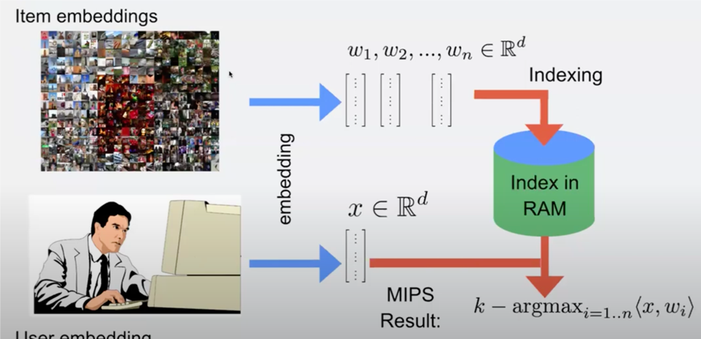
Embedding 可能来自于某个 embedding extractor，通常是一个神经网络，Encoder/Decoder 能把上游 Target 和目标连接起来，在读取的时候，可能希望有 vector index，能执行 ann 等查询，在满足一定预期的情况下拿到结果。

Faiss 是一个 Vector Searching Toolkit，包含 index, search, cluster, compress, transform vector 的内容。这里是希望根据 embedding 来直接做相关的搜索，并提供比较完善的处理链路。本项目最早由 facebookresearch 开始，但是最近还有 Vector 处理热潮，让这波东西能被更多人用上。Faiss 不会 extract features，也不是一个服务或者一个数据库，只是一个单机的 vector 处理库。

在 Faiss 上最基础的 workload 是 KNN 或者 ANN，用户提供一个 vector，然后拿到「最近」的向量，这个「最近」可以由向量的欧几里得距离来表示。

Performance axes of a vector search library

Vector Search 可能有下面的定义，比如说对于 Vector 查询最近的向量

对于给定的 database vectors :$\{x_{i}, i = 1..N\} \subset \mathbb{R}^d$ 和一个 Query vector $q \subset \mathbb{R}^d$, 搜索需要计算最近的一个向量。一个更常用的操作是 KNN，获取最近的 K 个向量。而还有一类搜索，对于给定的距离 $\epsilon$，找到小于这个距离的所有向量。这里面有几个讨论点：

Distance measures

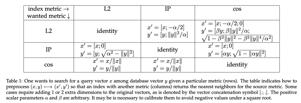
以上几种是最常见的距离，它们本身能够互相转换，但是如果是 Index 的话，很难根据一种距离定义的 Index 找到另外 Index 的搜索。

Brute force search

实际上，大部分精准 KNN 都需要暴力搜索，论文提到这个并不是 trivial 的

Implementing brute force search efficiently is not trivial [Chern et al., 2022, Johnson et al., 2019]. It requires

(1) an efficient way of computing the distances and

(2) for k-nearest neighbor search, an efficient way of keeping track of the k smallest distances.

(翻了一下代码，这块好像对应 IndexFlat::search )

某种意义上，这里会需要跟用户用提供的向量来计算距离，对于上述的距离，距离的计算实现方式可能会是：

• 自身 Batch 小的话直接 Scalar 或者并行的正常算
• 自身 Batch 大的话，可以用矩阵乘法类似的方式来计算，看代码里面有一些 exhaustive_inner_product_blas 这样的代码，分发到矩阵上来做计算

在处理 Knn 的时候，这里有多种 Pattern:

1. 如果只有一个，用 Top1 的方式来计算
2. 如果 k 的数量比较小，走 Binary Heap 来过滤
3. 如果 k 的数量比较大，去定义一个 reservoir 方式，这个有点类似 DB 的 Sort，先分组无序处理，超过一定阈值之后，会有一个 Resharp 流程，拿到一个临时的阈值，然后根据这个筛选

翻了下这块的代码，这里还是写的挺清楚的

template <class Consumer, class... Types>
typename Consumer::T dispatch_knn_ResultHandler(
        size_t nx,
        float* vals,
        int64_t* ids,
        size_t k,
        MetricType metric,
        const IDSelector* sel,
        Consumer& consumer,
        Types... args) {
#define DISPATCH_C_SEL(C, use_sel)                                          \
    if (k == 1) {                                                           \
        Top1BlockResultHandler<C, use_sel> res(nx, vals, ids, sel);         \
        return consumer.template f<>(res, args...);                         \
    } else if (k < distance_compute_min_k_reservoir) {                      \
        HeapBlockResultHandler<C, use_sel> res(nx, vals, ids, k, sel);      \
        return consumer.template f<>(res, args...);                         \
    } else {                                                                \
        ReservoirBlockResultHandler<C, use_sel> res(nx, vals, ids, k, sel); \
        return consumer.template f<>(res, args...);                         \
    }

    if (is_similarity_metric(metric)) {
        using C = CMin<float, int64_t>;
        if (sel) {
            DISPATCH_C_SEL(C, true);
        } else {
            DISPATCH_C_SEL(C, false);
        }
    } else {
        using C = CMax<float, int64_t>;
        if (sel) {
            DISPATCH_C_SEL(C, true);
        } else {
            DISPATCH_C_SEL(C, false);
        }
    }
#undef DISPATCH_C_SEL
}

库的 Python Wrapper 里面也提供了 knn 和 knn_gpu 这样的 wrapper。

Knn 有个很显而易见的毛病，就是这个算法完全不 Scalable，为此，实际上大家很多时候可能更倾向于 ann 做一些模糊的查询

Metrics for Approximate Neighbor Search

在 ann 中，用户接受不完美的结果，这给更符合需求的设计提供了空间。这里搜索来源于几个点：

(1) how well the distance metric correlates with the item matching objective and

(2) the quality of ANNS

对于第二个问题：

Ann 的 Accuracy 被称为 “n-recall@m”，表示在实际的 “n” 个最近中返回了 “m” 个

而对于 range-search，这里有 $\epsilon$和搜索时的允许的 $\epsilon^{'}$，允许的 $\epsilon^{'}$越大，搜索的结果会越多。

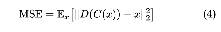
对于 distance metrics, 这里对于一个 Encoder C 和一个 Decoder D，有下面的衡量方式( MSE )：

这里也有一些资源的需求：

对于 Searching，有：

1. Search time
2. Memory usage
   1. constant memory overhead -> 结构的开销
   2. vector memory overhead -> 存储中对应的 vector 带来的边际开销
3. (for io) number of I/O operations (IOPS).

对于 Index Build(Training), 有:

1. index building time
   1. Training time
   2. addition time per vector
2. (for io) number of I/O operations (IOPS).

关于这些东西的 tunning 也是一个 Trade off。准确的说，这里大概有几个：speed, memory usage, accuracy，这三个。

Exploring search-time settings

这节介绍调优的内容还是非常有趣的，对于 Vector Index 通常会有一个或者多个 hyperparameter，作者表示，对于 speed / accuracy / memory usage，应该只保留 Pareto-Optimal 的参数，即定义上 Pareto Frontier 上的参数。

这里可能会需要一个多个参数组的笛卡尔积，但是 Faiss 因为对参数有先验知识，定义了一些剪枝的方式，来快速求出参数空间的保留参数集合。

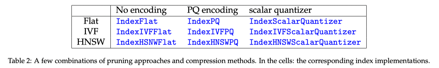
在实验中，这里还拆分出了不同的配置：

• 不同的 index 用不同的处理方式
• Compression ( 即 Vector 的有损编码等）

Refining ( IndexRefine )

Refine 这里会需要组合一个更快的 inaccurrate index 和一个准确率更高的 index。这里会先在更快的 index 拿到一组结果，再去慢的 index 精确计算这里面符合需求的数据。

This requires the accurate index to store the vectors in a way that allows efficient random access to possibly-compressed database vectors. Some implementations use a slower storage (e.g. flash) for the second index

Refine 这个代码也写的贼清楚：

/** Index that queries in a base_index (a fast one) and refines the
 *  results with an exact search, hopefully improving the results.
 */
struct IndexRefine : Index {
    /// faster index to pre-select the vectors that should be filtered
    Index* base_index;

    /// refinement index
    Index* refine_index;

    bool own_fields;       ///< should the base index be deallocated?
    bool own_refine_index; ///< same with the refinement index

    /// factor between k requested in search and the k requested from
    /// the base_index (should be >= 1)
    float k_factor = 1;
    ...
 };

当然，这样两个 Index 也不是唯一的 Refine 方式，实际上，在同一个 Index 中也有类似的方式，先有一个准确度低的 Vector，再去 decompress 然后去做精细的. 学术界也提供了多种解决的方案。

Compression levels

（笔者注：这一张因为笔者这方面完全没有基础，看的非常痛苦，越后面的章节越痛苦，有的地方可能就简单带过了，假以时日希望本人懂这块之后能把这里相关的内容补全）。

这里的 Compression 并不是我们通用的 zstd 之类的无损压缩，而是 quanitizer 这样的压缩，把原本的 embedding 映射到一个更小的空间中。定义 quantizer 为：C: $\mathbb{R}^d \rightarrow \{i = 1..K\}$ ，和对应的 Decoder: $\{i = 1..K\} \rightarrow \mathbb{R}^d$，在这里，搜索的逻辑会变成:

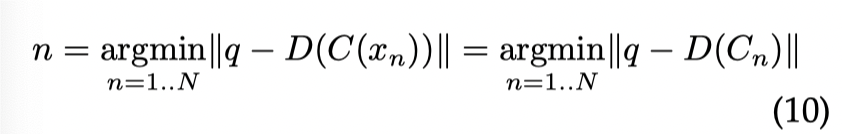
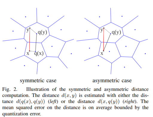
这里等价于，对索引的 index 做 quantizer，然后查询的时候等价于去 Decode 这部分数据，然后拿到这部分的最小值。这里还有个 asymmetric distance computation(ADC) 和 symmetric distance computation(SDC) 的区别（下图为 SDC)：

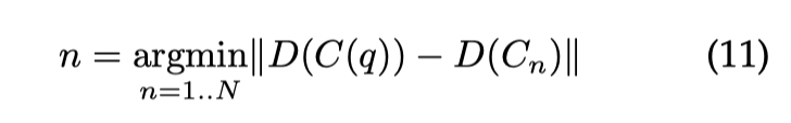
这里区别主要是 ADC 更精确，SDC 开销更小。Faiss 基本上采用的是 ADC:

Most Faiss indexes perform ADC as it is more accurate: there is no accuracy loss on the query vectors. SDC is useful when there is also a storage constraint on the queries or for indexing methods for which SDC is faster to compute than ADC.

The vector codes

理想的 Quanitizer 能最小化处理后 Vector 的 MSE, Kmeans 能比较好的做到这一点，K-means quantizer 将输入 vector 划分到 K 个 centroid，数据的表示在处理后需要$\lceil \log_{2}N \rceil$bits。这导致 k-means 在 accuracy 上很好，但是在 memory usage 和 encoding complexity 上，随着需要的 bits 增大而增大，Faiss 认为 k-means 实践上最好不要超过 3Bytes ( 即 16M）

Scalar quantizers

将向量的每个维度编码为一个 vector。这个比较典型的代码是对应的 IndexLSH，根据用户的向量输入，生成一组 threshold，然后按照大于或者小于 threshold

/*
 * dimension 0 corresponds to the least significant bit of b[0], or
 * equivalently to the lsb of the first byte that is stored.
 */
void fvec2bitvec(const float* __restrict x, uint8_t* __restrict b, size_t d) {
    for (int i = 0; i < d; i += 8) {
        uint8_t w = 0;
        uint8_t mask = 1;
        int nj = i + 8 <= d ? 8 : d - i;
        for (int j = 0; j < nj; j++) {
            if (x[i + j] >= 0)
                w |= mask;
            mask <<= 1;
        }
        *b = w;
        b++;
    }
}

ScalarQuantizer 有很多对应的模式，下面代码写的比较清晰，这里大概是把一个维度映射到 SQ{} 对应的位数上，来实现一个压缩。在压缩后，向量存储会按照下列模式进行：

The IndexRowwiseMinMax stores vectors with per-vector normalizing coefficients. The ranges are trained beforehand on a set of representative vectors.

/**
 * The uniform quantizer has a range [vmin, vmax]. The range can be
 * the same for all dimensions (uniform) or specific per dimension
 * (default).
 */

struct ScalarQuantizer : Quantizer {
    enum QuantizerType {
        QT_8bit,         ///< 8 bits per component
        QT_4bit,         ///< 4 bits per component
        QT_8bit_uniform, ///< same, shared range for all dimensions
        QT_4bit_uniform,
        QT_fp16,
        QT_8bit_direct, ///< fast indexing of uint8s
        QT_6bit,        ///< 6 bits per component
        QT_bf16,
        QT_8bit_direct_signed, ///< fast indexing of signed int8s ranging from
                               ///< [-128 to 127]
    };
    void train(size_t n, const float* x) override;
    
    /** Encode a set of vectors
     *
     * @param x      vectors to encode, size n * d
     * @param codes  output codes, size n * code_size
     */
    void compute_codes(const float* x, uint8_t* codes, size_t n) const override;
    
    /** Decode a set of vectors
     *
     * @param codes  codes to decode, size n * code_size
     * @param x      output vectors, size n * d
     */
    void decode(const uint8_t* code, float* x, size_t n) const override;
 };

Multi-codeblock quantizers

Faiss 支持 Multi-codeblock quantizers, 形式上这里可以当成有 M 个 Vector-quantizer，每个可以产生 K 个不同的 value。这里能够产生$K^M$ 个对应的 vector，然后 codesize 是$M\lceil \log_{2}K \rceil$

Product Quantizer (PQ) 把输入向量切分为多组，然后用 kmeans quantizer 独立处理每一组。对于 PQ6x10 的 product quantizer，它切分输入为 6 个子 vector，每个 10 bits (M = 6, K = 2^10 ).

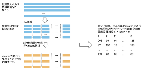
（这里参考了：ANN 之 Product Quantization - 名扬的文章 - 知乎 https://zhuanlan.zhihu.com/p/140548922 ，图片也来自这篇博文。）

Additive quantizers （加法量化器）是另一种 multi-codebook quantizer，这里可以当成 additive quantizer 由多个 sub-quantizer 组成，这里有两种：

• ResidualQuantizer：https://www.assemblyai.com/blog/what-is-residual-vector-quantization/

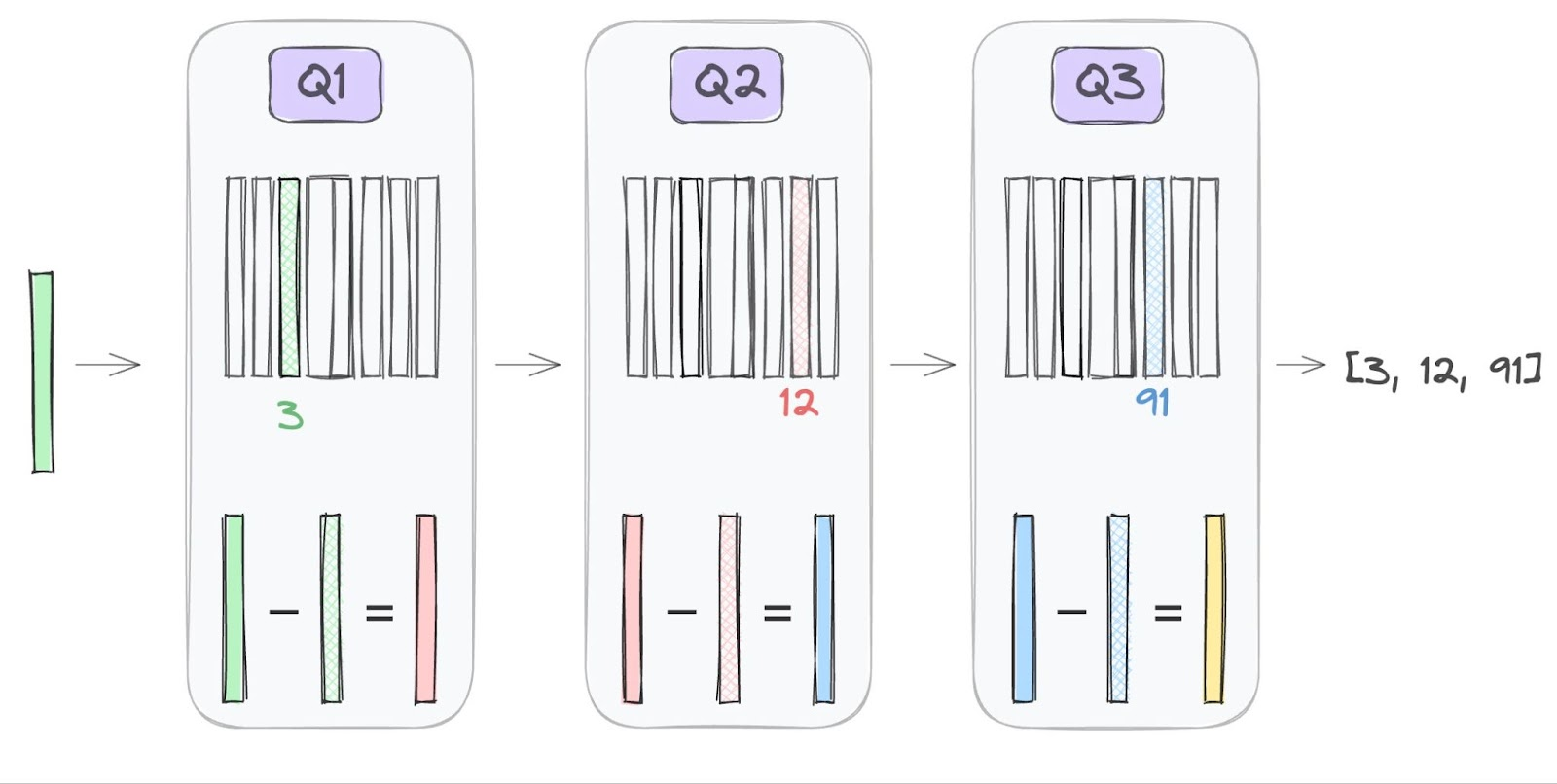
• Local search Quantizer: 从非 optimal 的地方做 Local Search，争取找到更优的结果（这个没找到我能看懂的资料，orz）

Faiss 还提供了混合 Quantizer，比如 PQ + Residual.

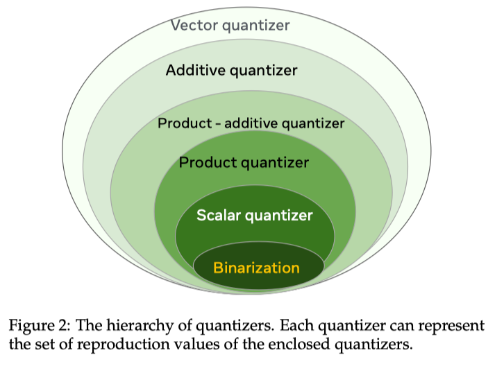
文章还提供了 Quantizer 的 Hierarchy, 这里的关键是下文：

The implications of this hierarchy are (1) the degrees of freedom for the reproduction values of quantizer i + 1 are larger than for i, so it is more accurate (2) quantizer i+1 has a higher capacity so it consumes more resources in terms of training time and storage overhead than i.

Vector preprocessing

To take advantage of some quantizers, it is beneficial to apply transformations to the input vectors prior to encoding them. Many of these transformations are ddimensional rotations, that do not change comparison metrics like cosine, L2 and inner product.

这里会做 PCA 之类的操作，尽量不改变目标 Metrics 的情况下，对输入向量处理。

Faiss additive quantization options

因为我看不懂 additive quantization，所以先跳过了。尴尬。。。

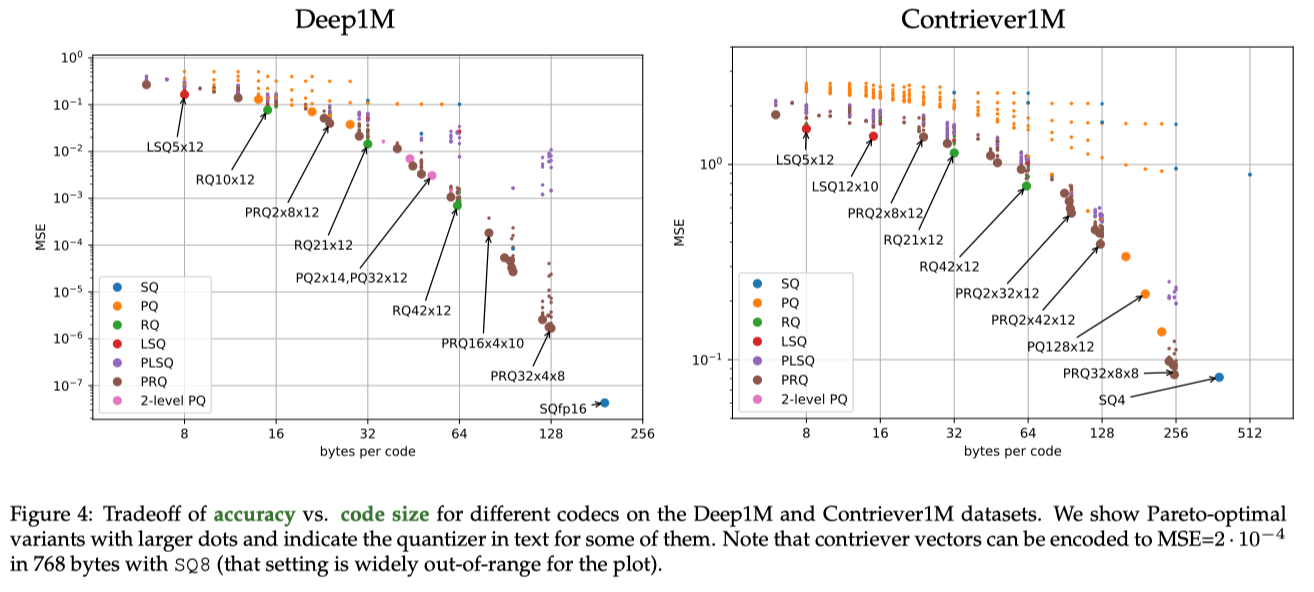
Vector compression benchmark

基本上等价于 code-size 大战 MSE 了

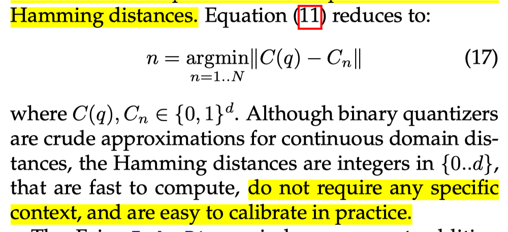
Binary indexes

用 binary quantizer + hamming distance 描述。

这里有一些相关的 Index:

• IndexBinary: Binary Quantizer Index 的基类
• IndexBinaryFlat: 暴力搜索 knn
• IndexBinaryIVF: 借助下一节的 IVF 来做搜索
• IndexBinaryHNSW: 用 HNSW 来做搜索
• IndexBinaryHash: 用前缀哈希来找到相关联的 bucket 并搜索

Non-exhaustive search

Non-exhaustive search is the cornerstone of fast search implementations for medium-sized datasets. In that case, the aim of the indexing method is to quickly focus on a subset of database vectors that are most likely to contain the search results.

比较早期的方法是 LSH，我们之前还贴过代码，这里的核心是把向量映射到 bucket 上，这里的问题是：

• 可能需要多个方向的映射，要不然很难找到关联的 bucket, 这里会增加 search time 开销
• 最早的方式并不 adaptive

Tree-based Index 也被提出，这里下层寻找有点类似 KD-Tree, 但是可能用的是 kmeans 的方式来找到下一层。

下面指出，这两种仍然是传统 db 的思路（索引结构）来做向量索引，这几种方式都不 scalable。向量的主要方式是 IVF 和 graph-based searching

Both in the case of LSH and tree-based methods, the hope is to extend classical database search structures to vector search, because they have a favorable complexity (constant or logarithmic in N). However, it turns out that these methods do not scale well for dimensions above 10.

Faiss implements two non-exhaustive search approaches that operate at different memory vs. speed tradeoffs: inverted file and graph-based.

Inverted files

IVF indexing is a technique that clusters the database vectors at indexing time. This clustering uses a vector quantizer (the coarse quantizer) that outputs $K_{IVF}$ distinct indices (Faiss’s nlist parameter). The coarse quantizer’s $K_{IVF}$ reproduction values are called centroids. The vectors of each cluster (possibly compressed) are stored contiguously into inverted lists, forming an inverted file (IVF). At search time, only a subset of $P_{IVF}$ clusters are visited (a.k.a. nprobe). The subset is formed by searching the $P_{IVF}$ nearest centroids, as in Equation (2).

以上这段直接摘抄原文了。即这里 build 的时候，根据 vector quantizer，来构成 nlist 个倒排，搜索的时候，这里会访问其中 P 个 ( nprobe )。

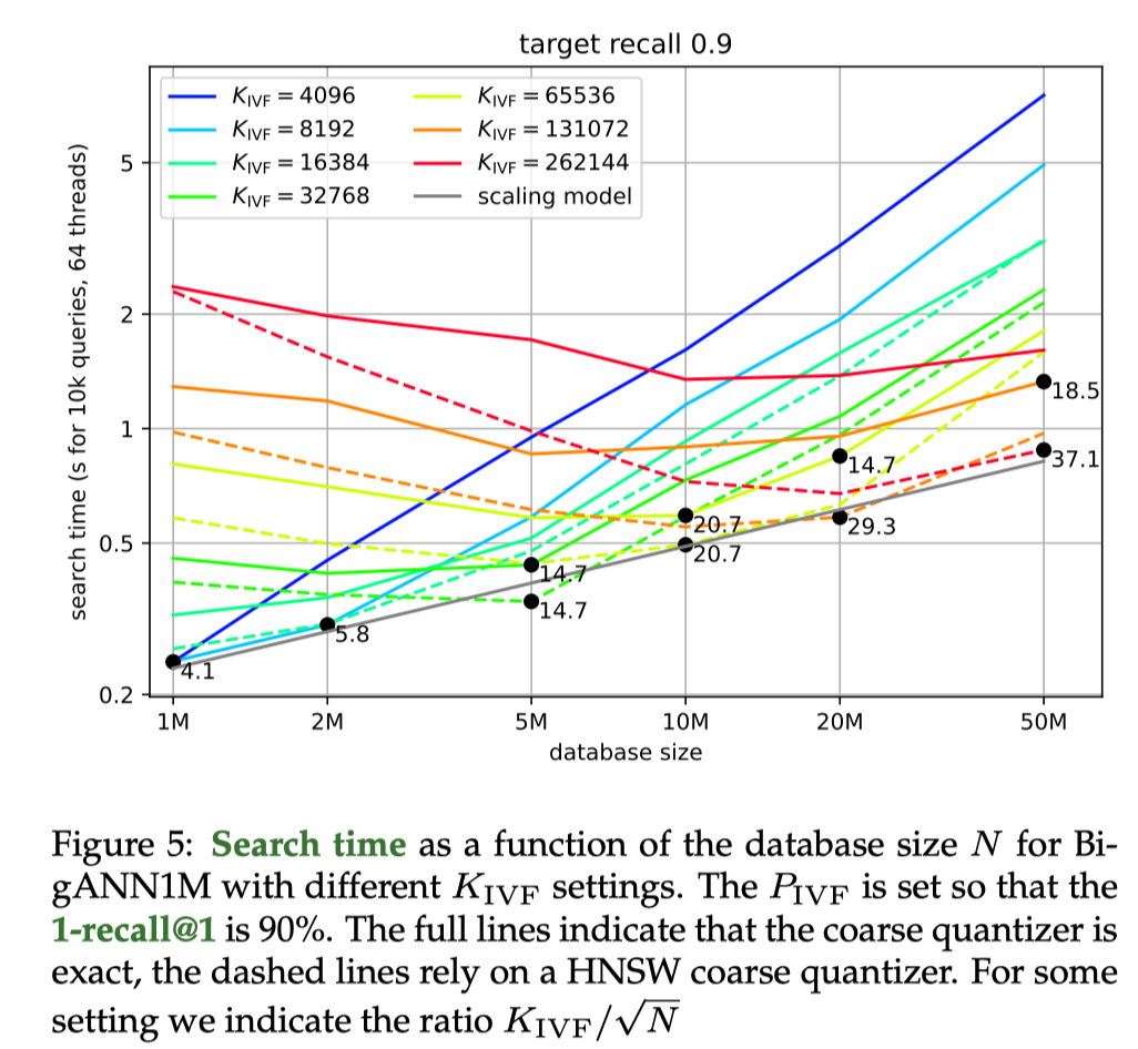
如果 nprobe 固定且 List 完全均匀，那么这里一次访问的计算距离如下（ 看意思是 IVF 需要全部访问）

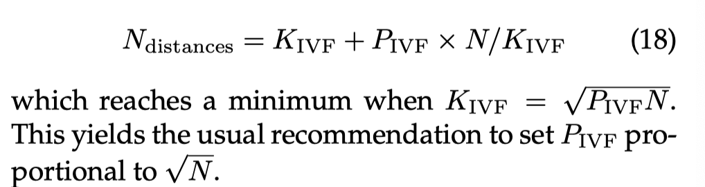
这里实际上是不准确的，因为：

• 随着插入，K 会增加，那么为了保证精准，P 也要增加
• 实际上 K 不一定会被全扫，如果 coarse quantization 是一个 hnsw 索引，那么可能只会粗筛选一些

这里还有很多特殊的优化，比如搜索大 batch 的时候做特殊优化，做特殊的 kmeans 等等。

Graph based

Graph based 本质上是一种通用的框架，它的建模大概是，Node 是指向 Vectors 的 Index （类似另一种形式的 IVF），在 search 的时候会需要在边上游走，找到最近的 Query Vector。这里可能就类似在图上游走的逻辑了，实际搜索可能会有类似 dfs bfs 的逻辑，search time 这样就会和搜索次数挂钩：搜索次数越多，搜索越准确和越慢

这里的代码会通常是个通用框架，作者认为某种程度上 tree-based search 和 IVF 是 Graph 的特殊形式，因为 Graph 本身可以看作对 Database Vector 临近关系的预处理。在这种图上直接尝试完整的 knn 并不合适，因为实际上一些搜索可能会陷入 local minima，所以这里建边可能也会有指向稍微远一点节点的边。大部分 graph 会使用一些固定的出边来方便平衡 search speed 和 memory usage，这样的话我们可以很好根据搜索的点、边来确定访问的内存开销（因为对于指定参数，你的访问点、边量大概也是可预测的）。

Faiss 中提供了 IndexHNSW 和 IndexNSG：

IndexHNSW

其中一些顶点（节点）被随机选择并提升为首先被探索的 Pivot。

本质上，这个有点像 SkipList，在构建的时候选取合适的地方连接起来，同时不让图陷入 local min。这里还要考虑精准度和内存占用，内存占用要加上出边的占用。

这个结构有个优点就是可以增量构建，就是可以动态插入 Vector

NSG

NSG 从输入的 kmeans 开始构建，并且将其中一些 short-range edges 替换成 longer-range edges。NSG 不使用多层，而是用 long-range edges 来搜索，并从固定的 center point 开始搜索。

因为 NSG 需要 KNN 图，虽有有一些特定的优化或者特殊构建方式（比如 NNDescent），但是这个相对来说 build 侧还是很耗时的。此外 NSG 是不允许动态更新的

Discussion

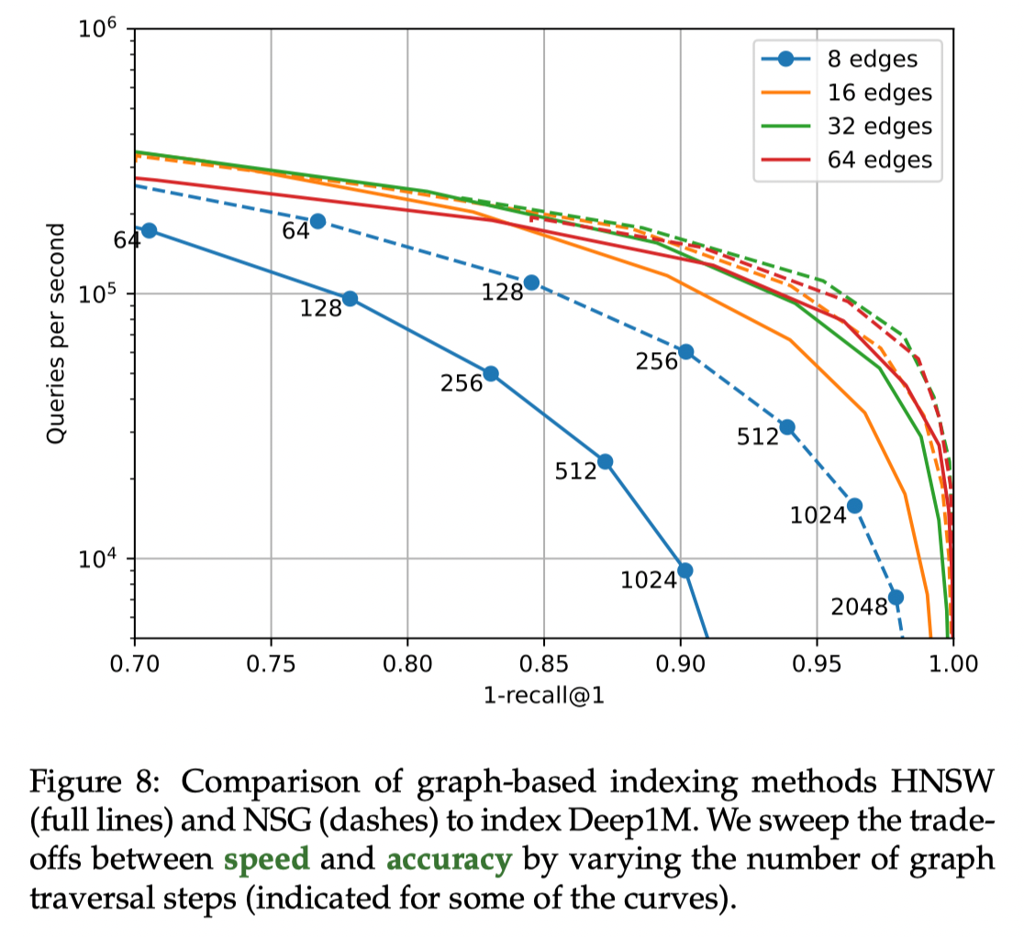
上述是 search time 的 trade-off ，关于 build 内容如下所述

Increasing the number of edges improves the results only to some extent: beyond 64 edges it degrades. NSG obtains better tradeoffs in general, at the cost of a longer build time. Building the input k-NN graph with NN-descent for 1M vectors takes 37 s, and about the same time with brute force search on a GPU (but in that case the k-NN graph is exact).

IVF vs. Graph-based

IVF Index 可以被看作 graph-based index 的特化版本，尤其是是当一个小的 graph-based index 被作为 coarse quantizer 的时候。在 Faiss 中，有下面的经验结论：

• Graph-based Indices 在内存没有过大约束，比如 1M index 以下的场景可以被使用。在 10M vector 以上，通常 construction time 会成为制约因素。
• 对于更大的 index，IVF 可能会成为仅有的选项，但是 IVF 前台可以挂一个 graph-based index 作为 coarse quantization 的优化项。

Reference

• Faiss paper: https://arxiv.org/abs/2401.08281
• SIGMOD’24 Vector Database Management Techniques and Systems: https://dbgroup.cs.tsinghua.edu.cn/ligl/papers/vdbms-tutorial-clean.pdf
• ANN 之 Product Quantization - 名扬的文章 - 知乎 https://zhuanlan.zhihu.com/p/140548922